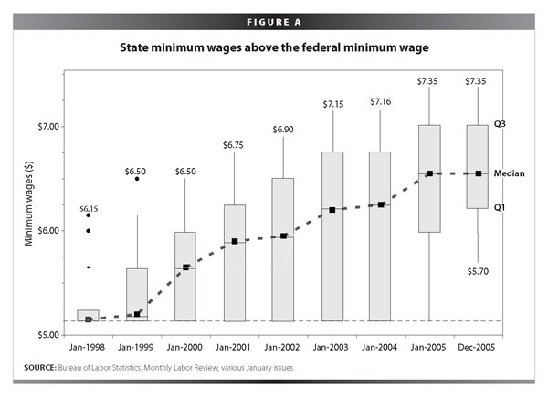
Although the federal minimum wage last rose in September 1997, minimum wages in the United States have not been static since then. Through the end of 2005, 17 states and the District of Columbia raised their minimum wages a total of 47 times. The list of these states includes both a border state, Delaware, and a southern state, Florida; all states north or east of Pennsylvania except for New Hampshire; the three states at the western edge of the Great Lakes; and the five states bordering the Pacific. Compared to the federal minimum wage of $5.15, the median minimum wage in these 18 states 1 had risen from $5.15 to $6.55 by December 2005; they ranged from $5.70 in Wisconsin to $7.35 in Washington State (Figure A ).

Have these state actions had any effect? Are wages higher than they would have otherwise been, i.e., are these higher minimums reaching their intended beneficiaries? Is employment worse than it would have otherwise been? The evidence presented here suggests that the answers are, respectively, yes, yes, and no. Wages are higher and employment is no lower in these states than they would have been without these actions:

• For teenagers, a group in which a large percentage of those employed earn low wages, there is strong evidence that minimum wage increases raise wages without reducing employment or discouraging labor supply.
• For young adults and adults with no college education, groups with smaller percentages of low-wage workers, there is some evidence that minimum wage increases lead to higher wages without reducing either employment or labor supply.
• Because of the small numbers in the sample, any results for racial minorities may well be weak. That said, results for racial minorities are mixed. One analysis provides evidence that the minimum wage may increase both employment and labor force participation of young African Americans (16-24 years old). The other analysis provides evidence (which further examination reveals not to be robust) that higher minimum wages reduce employment and labor supply among young Hispanics (16-24 years old).
• In the restaurant industry, often thought to be unusually sensitive to the minimum wage, the evidence is clear that minimum wage increases positively effect wages; one analysis finds a small positive impact on employment.
  • The evidence for any employment response exists in only a few cases, many fewer than for wages. In most of these,
  • the employment response is positive rather than negative, contrary to the old textbook explanation of the minimum wage. These and other factors suggest that a more careful look is called for in these cases.
• This more careful look indicates that evidence for both the positive employment response in the restaurant indus-try and the negative response among young Hispanics is not statistically robust. Only two employment responses survive this examination, those among teenage boys and among adult men whose education ended with their high school graduation. Both of these responses are positive.

The results come from two different statistical models applied to annual figures for each state constructed from the Current Population Survey (details of the survey are provided below). The focus of the analysis is on teenagers (16-19 years old) and young adults (20-24 years old). Low-wage workers are a large share of the workers in each of these groups. Results are also included for two groups of prime-age adults (25-55 years old): adults whose education ended before completing high school, and those whose education ended with their high school graduation. Although a majority of those affected by minimum wage increases are adults, a relatively small share of even these adult populations are affected. Any effects of the minimum wage on these populations will, thus, be harder to detect.

The next two sections explain the overall research strategy used in this paper and introduce the statistical models used to analyze the minimum wage’s effects. The section that follows describes the data. Only then do we come to results of the analysis, but before looking at the employment response it is necessary to consider the effect on wages. If wages do not respond to increases in the minimum wage in a measurable way, the cost to employers will not rise and thus we would not expect any adverse effects. The next two sections present results first for wages and then for employment of teenagers, young adults, and the two groups of adults by schooling. The two sections following present results for racial minorities and the restaurant industry. These are followed by the use of robust regression techniques to examine whether the statistically significant employment and labor supply results that have been presented are robust or fragile. The final section presents a summary and conclusion.

I. Research strategy

The most compelling arguments for the minimum wage appeal not to economic efficiency but to decency and fairness. The opposing arguments with the most traction assert that the loss in economic efficiency most hurts those whom the policy is intended to help. The debate about the minimum wage in both the policy arena and among economists has ended up focusing on costs and benefits. The benefits are higher wages and incomes for those at the bottom of the labor market, while the potential costs are job losses among these same workers. Thus, most research has examined whether minimum wage increases are causally linked to job losses.

Establishing the existence of costs has proven to be difficult. Large parts of the labor market, those with sufficiently high skills and wages, are widely considered to be insensitive to the minimum wage, at least at the levels within American experience. The limited reach of the minimum wage explains the common practice of beginning analysis by identifying vulnerable segments of the workforce, which are thought to include demographic groups with low skills and low wages; industries with a large number or a large proportion of low-wage workers; and regions where the minimum wage is high relative to the cost or standard of living.

To examine the costs and benefits of the minimum wage for its intended beneficiaries, we focus primarily here on four demographic groups. The first two are teenagers and young adults. At this age, work experience is usually slight, and few have had much chance to develop skills and work habits that would enable them to command high wages. Unshielded from any adverse employment effects of the minimum wage, teenagers and young adults are considered un-usually susceptible to employment losses in the face of minimum wage increases. Because reason also exists for concern about prime age adults without advanced education, we also consider adults with less than a high school education and adults whose highest level of education is high school.

For the same reasons we examine the experience of young African Americans (non-Hispanic) and young Hispanics (16-24 years old). Finally, we examine an industry, eating and drinking establishments, that is widely considered to be sensitive to minimum wage legislation because most employment consists of unskilled labor. Data on both this industry and the racial groups present some problems related to sample size, which are discussed below.

II. Statistical models

The data for this study are drawn from the Current Population Survey (CPS), conducted monthly by the Census Bureau for the Bureau of Labor Statistics. The CPS includes abou
t 50,000 households each month and asks for information on each member. A quarter of households, those belonging to a subgroup called the outgoing rotation group or ORG, supply more detailed information about employment and labor supply. The data used in this study are taken from house-holds in the ORGs and aggregated to the level of state and year. That is, each observation in this study consists of a set of averages or other measures calculated for a state over 12 months of ORGs. The CPS data are combined with information about each state’s minimum wage that was compiled separately.

Difference-in-differences
Examination of data only from states that raised their minimum wage might produce misleading results, since wages and employment can vary for many reasons other than the minimum wage. Based only on data from these states, inferences that wages rose or employment fell due to a minimum wage increase could easily be mistaken. The difference-in-differences technique is perhaps the simplest and certainly one of the most common techniques for avoiding this problem when examining policy interventions. It is a technique that parallels the experimental paradigm for medical trials.

In a medical trial, if all individuals in the trial received the drug being tested, its actual value would be hard to gauge. Some will improve naturally without the drug, while others may never improve or get worse even if the drug has medical value. The solution is to assign people in the trial randomly to one of two groups, experimental or control. Before the assignment, the participants may be closely matched on a variety of factors thought to be relevant so that each group contains similar numbers of each type. Those in the experimental group receive the medication according to a well-defined protocol, and those in the control group do not. In many trials, due to concern about the placebo affect, members of the control group receive a fake treatment, paralleling the experimental protocol except in ways that are relevant to the trial. As a result, people in each group are not sure about the group to which they belong. These precautions ensure that any difference in outcomes between the two groups is almost certainly due to the drug in question. By comparing the outcomes of the two groups, how many in each group improve, how many in each get worse, and how many show no change at all, it is possible to determine the minimum and maximum effects of the drug.

In few analyses of social policy is it possible to effect this degree of matching, randomization, and participants’ ignorance of the treatment. The difference-in-differences technique is an attempt to mimic this methodology as closely as possible. It involves first dividing the observations along two dimensions. In one, observations are identified as belonging either to the experimental group or the control group. The experimental group in the case at hand is states that raised the minimum wage between 1998 and 2005, while the control group would be the remaining states. The other dimension is the time periods before and after the policy intervention. With the federal minimum wage rising in 1997, and the focus being rises in state minimum wages since then, the before period can be no earlier than 1998. The data available for this analysis prevent the after period from being later than 2005.

Ideally, the control and experimental groups are otherwise closely matched so that the only important difference is the policy intervention. Often, especially with observational (rather than experimental) data, the two groups differ in important ways. That is the case with this analysis. States differ from each other in ways other than whether they’ve raised the minimum wage.

One solution is to recast the difference-in-differences technique through regression, a technique that attempts to determine the relationship between one or more dependent variables, in this case wages or employment, and a predictor variable—a minimum wage increase. With regression, one can include control variables that capture the dimensions along which the experimental and control groups must resemble each other. In this way, the two groups, control and experimental, are brought more closely into alignment except for the policy intervention, the minimum wage increase. 2, 3

Panel regression
The difference-in-differences framework has a weakness with respect to the data analyzed here. In the clinical test example described above, the time span is easily divided into three periods, before, during, and after. The drug is administered in a well-defined and consistent way to trial subjects in the second period, and the statistical analysis is applied in a well-defined and consistent way to measurements made in the other two periods. In analyses of social policy that rely on difference-in-differences, this clean division of time periods is also desirable. Here that is not possible.

The federal minimum wage rose in September 1997. Two states, Vermont and the District of Columbia, raised their minimum wages one month later, to $5.25 and $6.15, respectively. Oregon and California raised theirs early in 1998, to $6.00 and $5.75, respectively. These four states were so fast out of the gate that it is difficult to define a before period that excludes the 1997 federal minimum wage increase, which affected states in both the experimental and control groups. At the other end of the period, 11 states increased their minimum wages in 2005, six in January; one each in May, June, and August; and two in October. Finally, states raised their minimum wages a different number of times, by different amounts, and at different moments. Nothing resembling a well-defined protocol exists.

An alternative analytic technique is panel regression, similar but not identical to the regression in the difference-in-differences analysis. The similarity is due to use of the same dependent variable and the same control variables. The differences come from using all the periods rather than just those designated before and after, and from augmenting the list of control variables. The most important addition is including the minimum wage itself in the list. This allows us to differentiate among states that made small, medium, and large changes, and states that made one change from those that made many.

Finally, because of the large number of observations, variables can be added that control for stable, unmeasured influences within each year and each state without destroying the possibility of detecting an effect of the minimum wage increases. The structure of the panel analysis makes it possible to correct explicitly for the lack of a well-defined protocol. It controls for differences across the minimum wage states in the size of minimum wage increases, in the number of minimum wage increases, and in the timing of minimum wage increases.

The two analyses, difference-in-differences and panel regression, measure different phenomena. The former estimates the average change in the dependent variable (a wage measure, the employment ratio, or the labor force participation rate) in the minimum wage states in 2005 due to increases in the minimum wage in those states over the period 1998-2005. That is, it answers the question, “How different is the dependent variable in these states from what it would have been if the minimum wage had remained at its 1997 level?” Panel regression instead asks more directly, “How does the dependent variable respond to the minimum wage?” The structure of this analysis makes it straightforward to transform the estimates into a traditional economic measure, the elasticity, complete with 95% confidence intervals t
hat allow us to evaluate the statistical significance of the figure. 4

III. A look at the data

Many factors other than the minimum wage can lead to different labor market outcomes, including characteristics of both prospective workers and prospective employers. This is why both statistical techniques above rely on regression analysis, since it easily allows for variables that control for these other factors. Are these control variables important, or is simpler technique possible? To answer that question, we need to examine how the different groups in the minimum wage states, those that raised their minimum wages during the years 1998-2005, compare with counterparts in the non-minimum wage states, states that did not. 5 Consider the younger workers first, teenagers and young adults. The minimum wage states have higher levels of both enrollment and schooling. Racially, they are less white, and, among young adults, more Hispanic. Proportionately, they have fewer native-born citizens and more foreign-born citizens and non-citizens. In the minimum wage states, larger fractions of teenagers and young adults live in metropolitan areas. Fewer are married-living-with-spouse and more are other marital status. A smaller proportion of young adults in the minimum wage states live in households with very low incomes. Larger fractions of both age groups in the minimum wage states live in the most affluent category of households. The magnitudes of these differences suggest that control variables at worst are unnecessary, and will likely make results more reliable.

Bound workers
What about the workers most likely to feel the effects of minimum wage increases? Bound workers are those who are employed in the minimum wage states in the year before a minimum wage increase, and whose wage at that time is less than what the minimum will be following the next increase. Because they earn between the current and the next minimum wage, employers must either raise their wages or lay them off after the next rise in the minimum wage. How do young bound workers compare to others of their own age group in the same (minimum wage) state but with higher wages? They are no less likely to be enrolled in school, but their level of schooling is less. Bound teenagers are more likely to be white and less likely to be either black or other; more likely to be native-born citizens and less likely to be either a foreign-born citizen or a non-citizen; and more likely to be living outside metropolitan areas. Bound young adults are less likely to be married-living-with-spouse, and more likely to be in other marital status.

One interesting point concerns gender and bound workers. The fraction of all workers in both the teenager and young adult age groups that is female is the same across the two set of states, 49% of teenagers and 50% of young adults. However, bound workers (who can be identified only in the minimum wage states) are disproportionately female in both age groups: 54% of bound teenagers and 57% of bound young adults. The differences between these figures and their own-state averages are statistically significant (at a 5% level).

With regard to family income, bound teenagers are no different from other teenagers in their state, but bound young adults are more likely to be living in low-income households and are less likely to be from households in the most affluent category. This last point suggests that, if the minimum wage can increase earnings of bound young adults and not harm their employment prospects, it would serve a useful purpose.

Adults with no college education
Lower proportions of adults with less than a high school education (adults-LTHS) in the minimum wage states are Hispanic, and higher proportions are both white or black. Adults with a high school education (adults-HS) exhibit a similar pattern, except that the difference for whites between the two groups of states is not statistically significant. Residential patterns are similar for both groups, with more living outside central cities but within metropolitan areas in the minimum wage states, and fewer entirely outside metropolitan areas. Adults-LTHS are less likely in the minimum wage states to be married and living with spouse, and more likely to be in other marital status. Adults-HS are more likely to be married and not living with spouse in these states, but the absolute numbers are tiny. The distribution of family income is more bimodal in the minimum wage states for both sets of adults primarily because those states have substantially more in the lowest income category and correspondingly fewer in each of the intermediate categories.

Wages and employment, labor supply, and unemployment
In testing for a wage response to a minimum wage increase, it is necessary to choose a wage measure likely to reveal this impact, if it is present in the data. Obvious candidates include the average wage, perhaps the average of the logarithm of the wage (to correct for skewness in the underlying distribution) and the median wage. Because they are generally too high up the wage scale to be moved by changes in the minimum wage, they are not the best choices. Thus, while looking at these three, we focus on two that are further down the scale, the 30th percentile, and the average wage of those earning less than the median wage, in the expectation that they are more likely to pick up a minimum wage effect.

For both groups of younger workers, all measures of wages are higher in the minimum wage states during 1998-2005. For adults-HS, this disparity is less clear, since at the bottom of the distribution the difference is not statistically significant. There are no statistically significant differences for adults-LTHS between the two sets of states for any of the wage measures.

Having considered wages, the next question is, what other variables should be considered? The employment ratio (also referred to as employment), the proportion of the population or demographic group that is working, is an obvious choice. Presumably, anyone working before a minimum wage increase would be willing to work afterward. Either the increase has no effect on their wage, leaving them no better or worse off, or their wage rises, in which case they should be even more willing to work than before. If employment declines as a result of a higher minimum wage, it is reasonable to assume that people were laid off involuntarily.

The labor force participation rate (LFPR, or labor supply) may be a better gauge of how the minimum wage affects people’s welfare. 6 If employment declines due to a higher minimum wage, those effected by the minimum wage, either through job loss if previously employed or a lower probability of finding work if not, can choose not to be part of the labor force. If they do not make this choice, if instead LFPR increases following a minimum wage increase, the implication is that the prospect of a smaller probability of finding a job in exchange for a higher wage is a reasonable trade-off. If the LFPR rises, then the minimum wage has improved the welfare not only of those employed after the increase but also of those in the labor force but unemployed after the increase.

In the minimum wage states employment is lower for all but young adults. Labor supply is lower for all groups but adults-LTHS. Unemployment rates show no statistically significant differences for younger workers, but are higher for each of the adult groups in the minimum wage states.

As a large and growing literature has shown, the actual impact of minimum wage increases is an empirical question. The next section presents results from the two different statistical me
thods to gauge the impact of recent changes in state minimum wages on the earnings and employment of affected workers.

IV. Effect on wages

Difference-in-differences estimates
Table 1 shows results of the difference-in-differences analysis for wages. All the estimates for “All teens” are positive, and all but that for the logarithm are statistically significant. For teenage girls, all the estimates are positive and statistically significant. For teenage boys, all are positive, but only one is statistically significant, that for the average wage of those earning less than the median. Teenagers in the minimum wage states, especially teenage girls, had higher wages in 2005 than they would have had without the minimum wage increases.

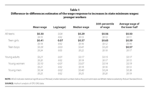
The average minimum wage in the 18 states of the experimental group was $1.40 higher than the federal minimum wage by the end of 2005. The first number of the first row in Table 1 indicates that the mean wage for all (working) teenagers in each of the minimum wage states was $0.30 higher (more or less) in 2005 as a result of the minimum wage increases. According to the third number in the same row, the median wage for all teenagers was $0.29 higher on average in the minimum wage states in 2005 than it would have been otherwise. The bigger numbers in the last two columns show that the impact of the minimum wage increases was generally even greater toward the bottom of the wage distribution. The 30th percentile of teenage girls’ wages was $0.65 higher, and the average wage of teenage boys was higher by almost as much, on average, in the minimum wage states.

The lower half of Table 1 indicates that, according to this analysis, young adults’ wages display no statistically discernible response to minimum wage increases. Results for adults-LTHS and adults-HS resemble those for young adults: no statistically discernable response, and several point estimates less than zero (details in Table A1). According to the difference-in-differences analyses, the minimum wage is associated with higher wages for teenagers but an effect is not discernable for adults.

Panel regression estimates
Table 2 shows elasticities calculated from the panel regression estimates. The calculations indicate a clear and strong response of teenage wages to the minimum wage. Elasticities (with respect to the minimum wage) of the mean wage, of the two percentile measures, and of the mean of the lower half are all greater than 1, and in several instances exceed statistically significant results for the median and the logarithm as well as the mean of the lower half.

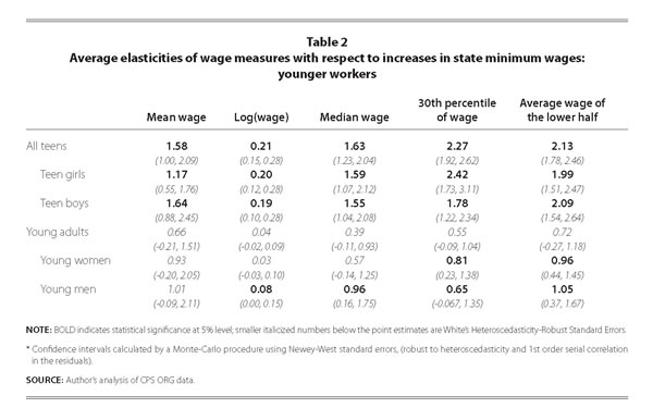
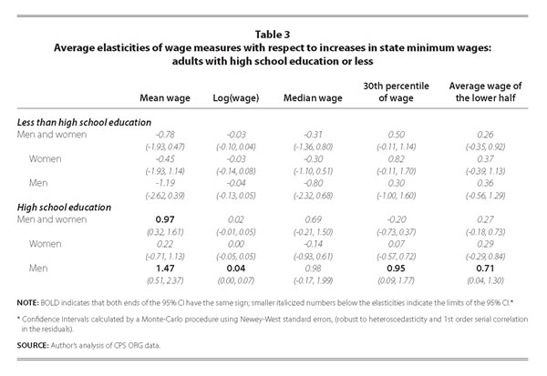
Table 3 shows the same elasticities calculated for the two adult groups under consideration. For adults-LTHS, none of the elasticities are statistically significant. All the point estimates are positive for the two measures most sensitive to the bottom of the distribution, and all are negative for the remainder. The results for adults-HS show a positive effect on wages. Elasticities for all measures of men’s wages are positive, and except for the median are statistically significant. Excepting the elasticity for the logarithm of the wage, they are also quite strong, though the CIs are fairly broad, which leads to some uncertainty about their precise size. The elasticity for the mean of men’s wages is so strong that the combined elasticity for men and women is significant and close to 1.

Both the difference-in-differences analysis and the panel analysis indicate that, in states that increased their minimum wages during this period, teenager’s wages were higher as a result, both during the period and by the end of it. The panel analysis provides evidence that the minimum wage also raises wages for low-wage young adults and some evidence that wages of adults-HS also respond to higher minimum wages, especially those of men in this group.

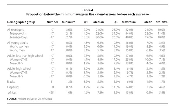
Does the lack of a finding of a wage response for some categories of adults mean that they do not benefit from the minimum wage? Not necessarily. Although teenagers are a smaller share of those affected by the minimum wage than are adults, a larger share of teenagers is likely to be affected by a minimum wage increase than are adults. This is true even of the subsets of adults examined, as can be seen in Table 4, which presents descriptive statistics for each demographic group of the percentage of bound workers in the calendar year before each minimum wage increase. On average, about 20% of teenagers were bound workers for these 47 minimum wage increases. The average percentages of bound workers for young adults and for adults-LTHS are roughly one-third as large, so minimum wage effects here are likely to be more difficult to discern. The percentages for adults-HS are about one-third again as large as the previous groups, so effects here are likely to be very difficult to discern.

The lack of evidence for a positive wage effect for adults is therefore likely the result of the difficulty in honing in narrowly on adults that are likely to be affected. This difficulty is why many studies of the minimum wage look only at teenagers or other groups that have high proportions subject to a minimum wage increase. Clearly many adults do benefit from an increase of the minimum wage, and more than the number of teenagers who do.

V. Effect on employment and labor supply

With the substitution of the employment measure for the wage variables, the difference-in-differences test for employment is identical to that for wages. 8 Comparing Table 5 with Table 1, the most striking pattern is that not one of the estimated effects for either teenagers or young adults is statistically significant: not for either variable, not for any age group or gender sub-group, and not whether the unemployment rate is included. With the adult male unemployment rate included in the regression, all of the point estimates are minuscule. In 2005, the employment ratio of all teenagers in the minimum wage states averaged 0.38, ranging from 0.15 to 0.56. According to the statistically insignificant point estimate, -0.007, the employment ratio might have been 2% (percent, not percentage points) lower in those states due to the minimum wage. Of course, according to the standard error it might reasonably have been anywhere between nearly 10% higher and 13% lower. Without the adult male unemployment rate in the regression, all point estimates are positive, and somewhat larger in absolute value, although the standard errors give us as much reason to pause as previously. This sign change suggests no need to be concerned that the unemployment rate might obscure the effect of the minimum wage, and strengthens confidence that the variable is useful as a business cycle control. The difference-in-differences estimates for labor supply are qualitatively similar.

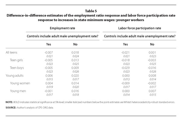
The difference-in-differences analysis of wages for the two adult groups found no discernible impact of the minimum wage. That is not quite the case for employment and labor supply. Labor supply of women-LTHS shows a statistically significant decline in response to the minimum wage. In the minimum wage states, the estimated minimum wage coefficient in the LFPR equation is -0.0
52, with a standard error of 0.026, according to the analysis that included the unemployment rate (see Table A4 for details). This finding is somewhat suspect given the lack of wage response, and the panel regressions do not confirm it.

The panel regression for these variables differs from the difference-in-differences analysis in an important respect from that for wages. Because inflation reduces the bite of the minimum wage, it is necessary to correct for this. In the analysis presented in Tables 6 and 7, the minimum wage has been adjusted by dividing through by the previous year’s value of the average wage for the lower half of each demographic group’s wage distribution. As wages at the bottom of the distribution rise, the minimum wage becomes less relevant, and is therefore less likely to have any effect on the labor market. This adjustment accounts for this. Use of the previous year’s value avoids underestimating the effect of a minimum wage increase, something that might occur from using the current year’s value, which is likely to rise in response to a minimum wage increase this year.

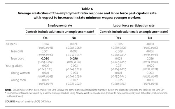
Evidence of a negative employment affect in Table 6 is even weaker than in Table 5. All the point estimates of employment elasticities for teenagers are positive. Furthermore, those for teenage boys are statistically significant. That is, there is evidence that employment of teenage boys rises in response to minimum wage increases.

There is no reason to look further at any of the other numbers in Table 6. All of them, both the employment elasticities of young adults and the elasticities of LFPR for both teenagers and young adults are statistically insignificant. While the point estimates of the employment elasticities are all negative, they are both statistically insignificant and very tiny. Those for labor supply are positive half as often as they are negative, and are somewhat larger in absolute value than the insignificant employment elasticities.

These groups, teenagers and young adults, were chosen because of suspicions that they were unusually vulnerable to adverse effects from the minimum wage. The overall impression from both tables is that employment during this period did not suffer from higher minimum wages. If anything, the minimum wage increased employment among teenage boys.

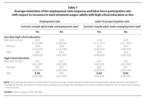
The corresponding elasticity estimates for the two adult groups appear in Table 7. They are slightly larger in absolute magnitude than those for younger workers (Table 6), but again are almost all statistically insignificant. The exceptions are employment and labor supply of men-HS. As with teenage boys’ employment, the minimum wage slightly raises not only employment but also labor supply of these men.

This lack of evidence for a negative employment result is quite striking, especially with respect to teenagers. Both statistical approaches found clear evidence that teenagers’ wages were higher as a result of the minimum wage. However, this appears to have had no adverse effect on teenagers’ employment. According to the panel analysis, low wages of young adults respond to the minimum wage, yet it is not possible to detect an adverse effect on their employment. Finally, there is no response of labor supply to the minimum wage.

VI. Racial minorities

It is possible that the demographic groups are too broadly defined to find an employment effect, although this is clearly not the case for wage effects. Other groups suggested to be disproportionately affected by minimum wage increases are racial minorities, specifically young African Americans (non-Hispanic) as well as youth of Hispanic descent. Examination of these two groups using the techniques of this analysis is difficult. A rule of thumb in using the CPS is that following aggregation (e.g., to the level of annual averages of state and year), averages should be based on no fewer than 75 individuals. Even with 50,000 households per month, or about 6,250 households per month in the two ORGs, few states have large enough samples of young African Americans or Hispanics over the course of a year to meet this criterion.

For African Americans, there were 21 states that consistently satisfied this criterion once the two vulnerable age groups, teenagers and young adults, and both genders were merged. Seven of these were minimum wage states, California, Delaware, the District of Columbia, Florida, Illinois, New Jersey, and New York, and 14 were not. For Hispanics, there were only 10 states, of which five were minimum wage states: California, Florida, Illinois, New Jersey, and New York were the minimum wage states; Arizona, Colorado, New Mexico, Nevada, and Texas were not.

A look at the data
Comparisons of both young Hispanics and young African Americans in the minimum wage states to their same-race counterparts in the non-minimum wage states as well as to whites in the same states are qualitatively similar until we get to money variables. 9 Young African Americans in the minimum wage states live in households with higher average family income than those in the other states. The situation is less clear for Hispanics, because the minimum wage states have higher proportions at both ends of the distribution.

Similarly, all measures of young African Americans’ wages are higher in the minimum wage states, but the only wage that is higher in these states for young Hispanics is the average wage. The average wage for young African Americans in the minimum wage states is 108% of that in the other states, and the corresponding figure for young Hispanics is 104%. Similar to the age-based demographic groups, employment and labor supply are lower in the minimum wage states. It is probably no surprise that the family income, wage, and employment and labor supply figures for both groups are lower than for whites, while the unemployment figures are higher.

As before, it is plausible that the higher wages and lower employment rates are due to the higher minimum wage. Is that the case? The bottom of Table 4 provides information about the distribution of bound workers among young Hispanics and African Americans. The numbers are surprisingly small. The average proportion of young Hispanic workers (in the five minimum wage states in this sample) who are bound by the minimum wage is roughly the same as for all young adults, about 7%. For African Americans, the numbers are even smaller, less than for any category of young adults, less than for any category of adults-LTHS. These numbers and the small number of states that have data available suggest the likelihood of inconclusive results.

Analytic results
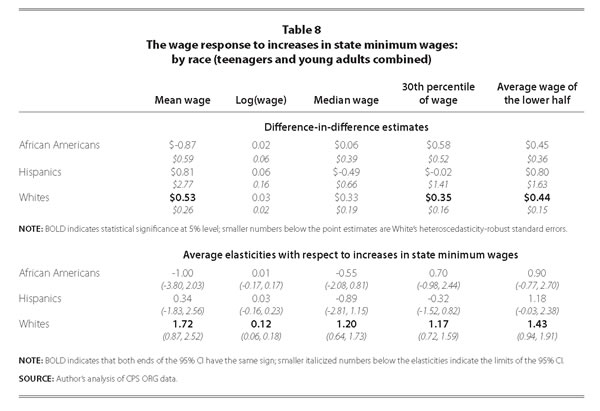
Table 8 displays the results for wages, including those for whites to provide a baseline.¹⁰ Both analyses, especially the panel analysis, show consistent minimum wage effects on wages of young white workers. The effect on the wages of either African Americans or Hispanics is not discernable.

The results for employment and labor supply that are shown in Table 9 are somewhat more interesting. The difference-in-differences analysis indicates that employment and labor supply of young African Americans increase in response to minimum wage increases, when the adult male unemployment rate is not included as a control. However, the results are sufficiently smaller when the business cycle control is included as to be statistically insignificant, and neither version of the corresponding panel analyses supports this result. More interesting are the employment and labor supply responses of young Hispanics when the
business cycle control is included: both, negative, though not strongly, at about -14%. With one exception, the remainder of the estimates in this table are both statistically insignificant and small.11, 12

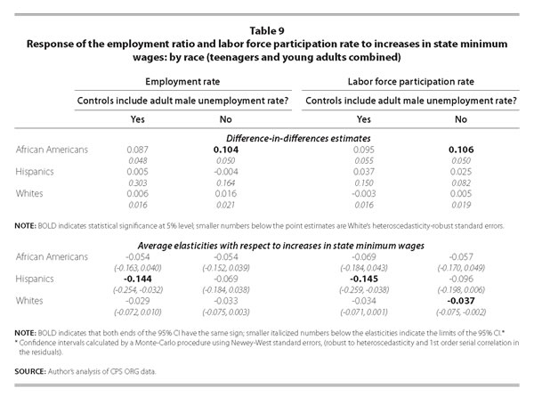
These results do not provide evidence of discernible benefits to minority youth. Does it harm them? Certainly not African Americans. The estimated impact on employment and labor supply of young Hispanics is negative, but as we show in section VIII, even this finding fails to stand up to closer scrutiny.

VII. Eating and drinking establishments

Restaurants and bars—eating and drinking establishments—are thought to be especially sensitive to the minimum wage. Whenever talk of raising the minimum grows, representatives of this industry warn that this will inevitably lead to employment losses. The federal law concerning the minimum wage sets a minimum wage for this industry half that of others, with the expectation that employees will make up the other half with tips. 13 Consequently, this industry is another common object of analysis in minimum wage research.

Analyzing this industry is difficult compared with analyzing the demographic groups because employment in the industry is a much smaller proportion of the population. In the survey that is the data source, some states and years have very small numbers of people employed in the industry. This can lead to a great deal of variation in estimates due only to random factors introduced by the sample. Consequently, not only is the reliability of the estimates more open to question; so is the reliability of the many different measures of wages at the bottom of the distribution that were considered above. Only two measures of wages are used here, the average wage and the average logarithm of the wage.

A look at the data
Workers in this industry are more than half female, 54% in non-minimum wage states vs. 52% in minimum wage states (a statistically significant difference). Differences in racial makeup of the work force reflect those we saw earlier when looking at teenagers and young adults; in the minimum wage states the makeup is less white and more Hispanic and other. It is also less black, a difference that is not statistically significant in the demographic groups examined earlier. The pattern of differences in citizenship is also similar, with fewer native-born citizens in the minimum wage states and more non-citizens and foreign-born citizens. This workforce is better educated in the minimum wage states, with a smaller proportion whose education ended before graduating from high school and a larger proportion at each level past high school. Compared to this industry in the non-minimum wage states, family income is higher. Wages average about $0.70 per hour more in minimum wage states, and employment in the industry averages about 1 percentage point of the population less, 8.9% vs. 9.8%. Both differences are statistically significant

Formal statistical analysis
To gauge the impact of the small samples, a problem mentioned previously, two sets of results are presented: for the whole sample, and for a restricted sample that includes only states that meet a minimum value, in all years examined, of people working in the industry who are included in the survey. The minimum here chosen is the median value of the sample used for each statistical procedure. For the difference-in-differences technique, 26 states (nine of which raised the minimum wage) have at least 55 people in the survey who are employed in eating and drinking establishments in both 1998 and 2005. For the panel analysis, 21 states (eight of which raised the minimum wage during these years) had at least 50 individuals in the survey employed in the industry in each year of the sample, 1998-2005.

Table 10 presents estimates of the minimum wage effects on the industry from both the difference-in-differences and the panel analysis. In the difference-in-differences analysis (top half of the table), both the full sample and the restricted sample exhibit evidence of the same pattern, a positive wage response and no employment response.¹⁴ In the full sample of states, average wages were $0.76 cents higher in the industry due to the minimum wage increases and in the restricted sample, $0.65 cents higher.

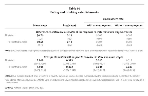
In the panel analysis, the results from both the full and the restricted samples clearly indicate that industry wages respond strongly to the minimum wage.¹⁵ In the full sample, the point estimate of the elasticity is nearly 3, with the bottom of the 95% confidence interval above 2. In the restricted sample, the point estimate is about 1.5, with the 95% confidence interval ranging between two-thirds and more than 2. When the adult male unemployment rate is included to control for business cycles, both samples indicate clearly that the response of employment is positive (and small). When the business cycle control is excluded, both point estimates of the elasticity decline a bit, with that in the full sample no longer statistically significant but that in the restricted sample remaining statistically significant

Together, these two analyses provide strong evidence that the minimum wage leads to higher wages in the restaurant industry and that the minimum wage need not hurt employment. The panel analysis suggests that industry employment may well respond favorably to the minimum wage. While counter-intuitive, it is consistent with other findings: not only Card and Krueger’s (1994, 2000) well-known papers examining New Jersey’s 1992 minimum wage increase, but also the more recent work of Dube, Naidu, and Reich (2006) that examines San Francisco’s legislating a minimum wage in 2004.

VIII. A second look at employment and labor supply

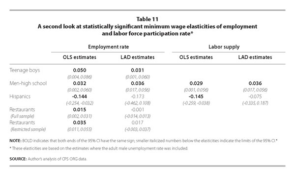
Few of the estimated responses of employment or labor supply to minimum wage increases are statistically significant, and most of these are positive. Table 11 shows the statistically significant employment and labor supply elasticities when the adult male unemployment rate was included in the regression ( labelled OLS estimates): employment of teenage boys, adult men who graduated from high school, and Hispanic youth and in the restaurant industry; and labor supply of men-HS and of Hispanics. 16

There are several reasons for taking a second look at these results. One is the overall paucity of significant results for these variables. A second is that these responses do not match up with the statistically significant wage responses. A third is the positive sign of nearly all of the point estimates. And fourth, the small samples underlying the results for Hispanics (only 10 states) and the restaurant industry (substantially fewer than 75 individuals underlying each observation, even for the restricted sample) suggest that a few unusual observations may be distorting the results.

A standard set of techniques, called robust regression, is commonly used to address this problem. One of the easiest to calculate is least absolute deviation (LAD). Conventional least squares regressions give a great deal of weight to outliers. LAD gives equal weight to all observations, so is less sensitive to outliers.

Table 11 presents LAD estimates of the elasticities in question, right next to the significant estimates already seen. The LAD estimate of the employment elasticity of teenage boys is a bit smaller, while the new estimates for both the employment and labor supply elasticities of men-HS are a bit larger than previously, but all remai
n statistically significant However, the LAD estimates of both the employment and labor supply elasticities of young Hispanics are no longer statistically significant, largely because the 95% CIs (or standard errors) are larger. In addition, the LAD estimates of the employment elasticities of the restaurant industry decline. The 95% CIs (or standard errors) both become smaller, and shift so that they now contain zero. The result is that the estimated elasticities for the restaurant industry are also not statistically significant

According to the robust regression analysis, the standard estimates of the employment and labor supply responses of young Hispanics and of the employment response for the restaurant industry are fragile. The most likely sources of this fragility are the small sample issues already mentioned: few states with sufficient representation in the CPS of young Hispanics and of people who work in eating and drinking establishments. This hypothesis is supported by the statistical significance in both analyses of the estimates in question for teenage boys and men-HS, both groups without the small sample issues.

IX. Conclusion

Between the last time the federal minimum wage was increased, in September 1997, and the end of 2005, 17 states and the District of Columbia raised their own minimum wages a grand total of 47 times. By the end of this period, the median minimum wage of these states was $1.40 (more than 25%) higher than the federal value. Examination of several demographic groups for which wages and employment are thought to be sensitive to minimum wages found some positive effect on wages and scant effect on either employment or labor supply. The same can be said for employees working in eating and drinking establishments.

For several reasons, the very few statistically significant employment and labor supply responses merited further attention. They did not match up with the statistically significant wage responses. With the exception of young Hispanics, where there appeared to be some evidence of adverse impacts on both labor supply and employment, all the statistically significant employment and labor supply responses were positive. About half of the statistically significant responses were in groups where there were already red flags around the issue of small sample size. Estimates based on least absolute deviation, a common robust regression technique, indicated that the estimates of both a negative impact on employment and the labor supply of young Hispanics and a positive impact on employment in the restaurant industry are fragile, most likely due to the small representation of both groups in the CPS sample. Overall, it is safe to conclude that statistically reliable evidence for any employment losses in the data is non-existent.

Due to the very large proportion of low-wage workers among employed teenagers, the effects on wages were clearest for this group. The effects on employment and labor supply were no clearer here than for any other group. Or perhaps a more accurate statement is that the wage effect was clearest, and the lack of any employment or labor supply effect was as clear for this group as for any other.

Economists examining the minimum wage often focus on teenagers, ostensibly because being low-skilled they are most vulnerable. The large proportion of low-wage workers is a related but not identical reason; it makes it more likely that if there are effects they will be recognized. The apparent lack of effects for other groups, especially wage effects, is most likely due to the small proportion of low-wage workers in these groups. The impact of the minimum wage on low-wage workers in these other groups is likely to mirror that of teenagers: higher wages and no employment or labor force response, certainly not an adverse one.

Among economists, the minimum wage and its impact on employment was unusually contested terrain during the 1990s. In a series of papers and a book, David Card and Alan Krueger presented much evidence that the minimum wage did not have adverse effects on employment, and a body of research by others supported their findings David Neumark and William Wascher presented much evidence contradicting these results, and they too had a body of research by others that supported their findings Much of the analysis on both sides considered datasets not previously examined, and often constructed especially for the specific analysis. The final volley between these two pairs was published in 2000, and much of the criticism on each side focused on the reliability of the datasets that the other pair had constructed.

In an attempt to answer the question once and for all, Card and Krueger repeated their most influential analysis on government data that provided a census of employment and earnings at all firms covered by unemployment insurance. The results of this authoritative analysis were qualitatively similar to the analysis that they had previously conducted on the smaller dataset: “The increase in New Jersey’s minimum wage probably had no effect on total employment in New Jersey’s fast food industry, and possibly had a small positive effect.” This appears to have been the final word in the ex-change. The results of the analysis in the present paper are consistent with those of Card and Krueger.

Though consistent with much work on the minimum wage conducted in the last 15 years, the results presented in this analysis are nevertheless surprising when viewed through the prism of a simple, textbook model of supply and demand. In this model, neither hiring nor firing imposes any costs on employers, and either all workers are identical, or employers can easily discern how productive potential employees are. As with all modeling assumptions, none of these assumptions is correct in reality. The results presented here indicate that the modeling assumptions are not merely useful simplifications. Rather, they impede understanding of labor markets, and the design of policy to affect them, both in general and specifically concerning the minimum wage, suffers. “Prism” is a less apt description of the simple textbook model in this context than “funhouse mirror.”

November 2006

Paul Wolfson is a statistical research associate at the Tuck School at Dartmouth College. The author would like to thank Jared Bernstein, Arindrajit Dube, Michael Ettlinger, Liana Fox, and Jesse Rothstein for comments on earlier drafts of this paper.